[머신러닝을 위한 파이썬] 15. Linear Regression - 4

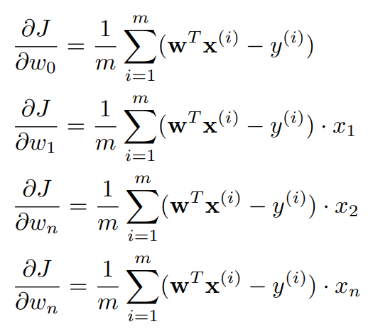
한 개 이상의 특성이 있을 때의 경사 하강법

한 개 이상의 특성이 있을 때의 경사하강법도 크게 다르지 않다. 일단 식은 다음과 같다.

코드를 작성하는 방법은 크게 두 가지가 있다. 첫 번째는 이중 반복문을 사용하는 것이다.

for _ in range(iterations):
    predictions = x.dot(theta)

    for i in range(theta.size):
        partial_marginal = x[:, i]
        errors_xi = (predictions - y) * partial_marginal
        theta[i] = theta[i] - alpha * (1.0 / m) * errors_xi.sum()
    
    theta_history.append(theta)
    cost_history.append(compute_cost(x, y, theta))

하지만 이중 반복문은 당연히 시간 복잡도상으로 좋지 않다. 다른 방법은 벡터화를 사용하는 것이다.

for i in range(0, num_iterations):
    hypothesis = x.dot(x, theta)
    loss = hypothesis - y

    cost = np.sum(loss ** 2) / (2 * m)
    gradient = np.dot(xTrans, loss) / m
    theta = theta - alpha * gradient

모델의 성능 평가하기

모델의 성능을 평가하는 방법에는 대표적으로 3가지가 있다.

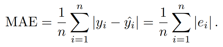
가장 먼저, Mean Absolute Error(MAE)이다. 이는 잔차의 ‘절댓값의 합’을 구한다. 공식은 다음과 같다.

코드 구현은 다음과 같다.

# 방법 1
np.abs(y - predictions).sum() / len(y)

# 방법 2
from sklearn.metrics import mean_absolute_error
mean_absolute_error(y, predictions)

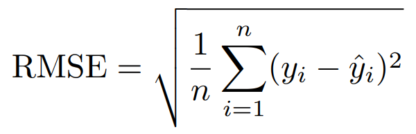
다음으로 Root Mean Squared Error(RMSE)가 있다. (간혹 제곱근을 하지 않기도 한다.) 공식과 코드는 다음과 같다.

# 방법 1
np.sqrt(np.mean((y - predictions) ** 2))

# 방법 2 - MSE 구하기
from sklearn.metrics import mean_squared_error
mean_squared_error(y, predictions)

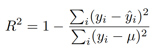
마지막으로 R-squared이다. 앞선 두 개 와는 다르게 1에 가까울수록(클수록) 좋다. 공식과 코드는 다음과 같다.

# 방법 1
1 - (np.sum((y - predictions) ** 2) / np.sum((y - y.mean()) ** 2))

# 방법 2
from sklearn.metrics import r2_score
r2_score(y, predictions)

Hold-out Method

데이터 셋을 train set과 test set으로 나누는 것을 ‘Hold-out Method’라고 한다. 데이터를 나누어야 하는 이유는 과대적합을 방지하여 모델의 성능을 높이기 위함이다. 각 set의 비율은 보통 train set 2: test set 1 정도로 하지만, 데이터의 양에 따라 달라진다.

from sklearn.model_selection import train_test_split
X_train, X_test, y_train, y_test = train_test_split(X, y, test_size=0.33, random_state=42)

별도의 출처 표시가 있는 이미지를 제외한 모든 이미지는 강의자료에서 발췌하였음을 밝힙니다.