
Credit Assignment Problem
An agent is hard to know which action was critical to the final result. Therefore, training an agent to choose the best action for each step is difficult. This problem is called credit assignment problem.
The simplest way to solve this is to add all rewards of each step after applying discount factor $\gamma$. The sum is called ‘return’. The following is an example of $\gamma=0.8$.
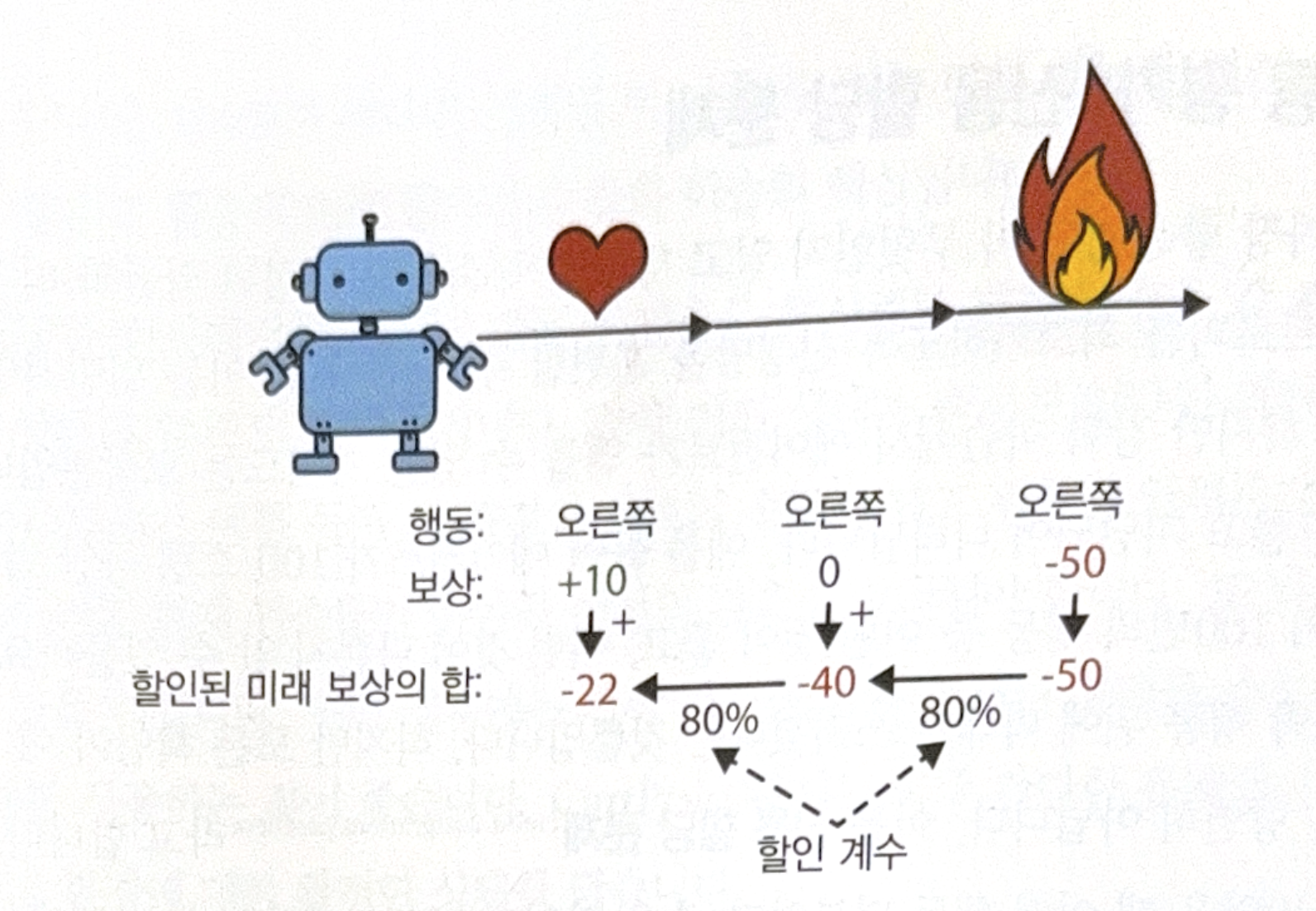
For example, at the first action, sum of discounted future reward is $10 + \gamma \times 0 + \gamma^2 \times (-50) = -22$. If a discount factor is close to 0, future reward will not be considered importantly. Reversely, if the factor is close to 1, future reward will be considered importantly.
We need to estimate how good each action is compared to the others. This is called action advantage. To do this, normalize all return of actions after many episodes. Negative value means bad action, and positive value means good action.
Policy Gradient
One of the most popular PG algorithms is REINFORCE algorithm. The process is as follows.
- NN policy plays a game multiple times. Calculate gradient that makes the action for each step have higher probability. Do not apply the gradient.
- After a few episodes, calculate return of each action.
- If a return of a action is positive, apply the gradient to have higher likelihood in the future. If negative, apply opposite gradient to have lower likelihood (multiply gradient vector and return).
- Average all gradient vector and perform gradient descent.
The following is a code implementation.
# Assume all action is good. Calculate gradient first, and apply after determining each action's return.
def play_one_step(env, obs, model, loss_fn):
    with tf.GradientTape() as tape:
        left_proba = model(obs[np.newaxis])     # print prob to left
        action = (tf.random.uniform([1, 1]) > left_proba)       # decide action by using prob. Go if false, go right if true.
        y_target = tf.constant([1.] - tf.cast(action, tf.float32))  # target prob.
        loss = tf.reduce_mean(loss_fn(y_target, left_proba))

    grads = tape.gradient(loss, model.trainable_variables)
    obs, reward, done, truncated, info = env.step(int(action))
    return obs, reward, done, truncated, grads


# play multiple episodes by using play_one_step
def play_multiple_episodes(env, n_episodes, n_max_steps, model, loss_fn):
    all_rewards = []        # save rewards
    all_grads = []          # save gradients
    for episode in range(n_episodes):
        current_rewards = []
        current_grads = []
        obs, info = env.reset()
        for step in range(n_max_steps):
            obs, reward, done, truncated, grads = play_one_step(env, obs, model, loss_fn)
            current_rewards.append(reward)
            current_grads.append(grads)
            if done or truncated:
                break
        all_rewards.append(current_rewards)
        all_grads.append(current_grads)
    return all_rewards, all_grads

# calculate the sum of discounted future rewards
def discount_rewards(rewards, discount_factor):
    discounted = np.array(rewards)
    for step in range(len(rewards) - 2, -1, -1):
        discounted[step] += discounted[step + 1] * discount_factor
    return discounted

# normalize
def discount_and_normalize_rewards(all_rewards, discount_factor):
    all_discounted_rewards = [discount_rewards(rewards, discount_factor)
                              for rewards in all_rewards]
    flat_rewards = np.concatenate(all_discounted_rewards)
    reward_mean = flat_rewards.mean()
    reward_std = flat_rewards.std()
    return [(discounted_rewards - reward_mean) / reward_std
            for discounted_rewards in all_discounted_rewards]

# some hyperparameters
n_iterations = 150
n_episodes_per_update = 10
n_max_steps = 200
discount_factor = 0.95

# optimizer and loss function
optimizer = tf.keras.optimizers.Nadam(learning_rate=0.01)
loss_fn = tf.keras.losses.binary_crossentropy

# train
for iteration in range(n_iterations):
    # calculate normalized rewards
    all_rewards, all_grads = play_multiple_episodes(
        env, n_episodes_per_update, n_max_steps, model, loss_fn)
    all_final_rewards = discount_and_normalize_rewards(all_rewards, discount_factor)

    # average gradients
    all_mean_grads = []
    for var_index in range(len(model.trainable_variables)):
        mean_grads = tf.reduce_mean(
            [final_reward * all_grads[episode_index][step][var_index]
             for episode_index, final_rewards in enumerate(all_final_rewards)
                for step, final_reward in enumerate(final_rewards)], axis=0)
        all_mean_grads.append(mean_grads)
    # apply gradient
    optimizer.apply_gradients(zip(all_mean_grads, model.trainable_variables))
Markov Decision Process
The following is a simple example of Markov chain.
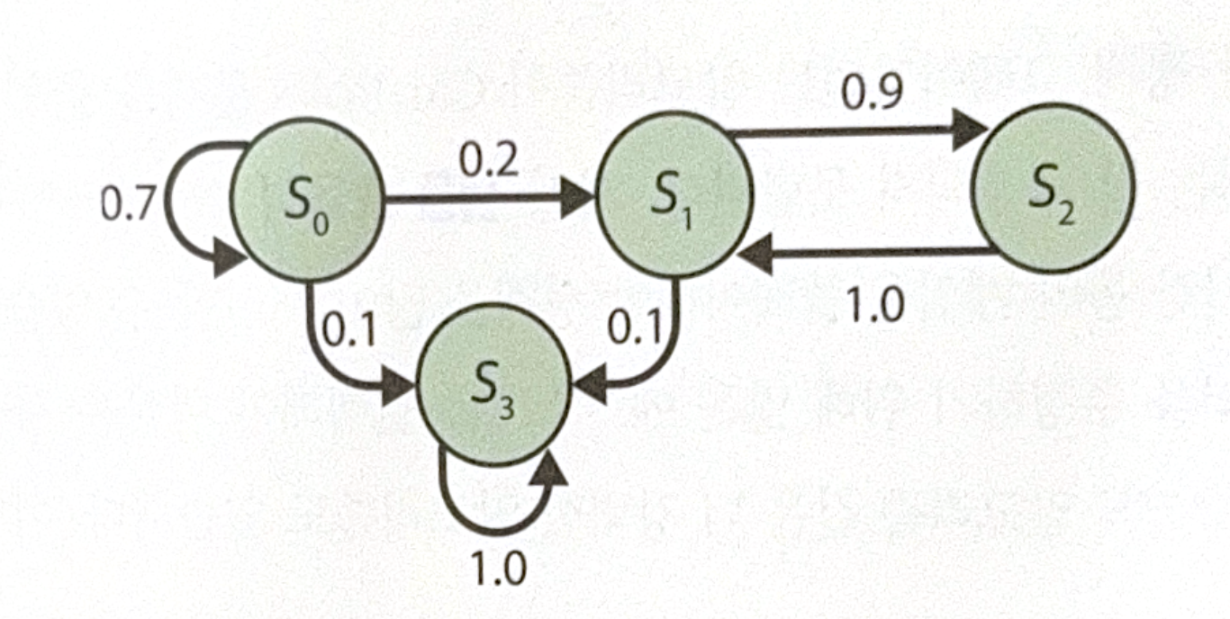
By using the chain, Markov Decision Process(MDP) was devised.

For example, let’s start at $s_0$. There are 3 choices, $a_0$, $a_1$, $a_2$. If we choose $a_0$, we will get +10 reward by the probability of 0.7. If we go to $S_1$, there are 2 choices. Going to $S_2$ is bad in the short term,(-50) but it could give us +40 reward one step later. Therefore, it is unclear which way to choose if we are at $S_1$.
Richard Bellman, who devised MDP, found the solution to estimate ‘optimal state value’ $V^*(s)$ of a certain state s. The value is a sum of discounted future return by assuming an agent will act in optimal at state s. If the agent act in optimal, Bellman optimality equation can be applied.
\[V^*(s) = \underset{a}{max} \displaystyle \sum_{s'}{T(s, a, s')[R(s, a, s') + \gamma \cdot V^*(s')]}\]- $T(s, a, s’)$: Probability of state s to s’ if an agent choose action a.
- $R(s, a, s’)$: Reward of state s to s’ if an agent choose action a.
- $\gamma$: Discount coefficient.
First initialize all state value as 0. Then, update them by using value iteration algorithm as a following formula.
\[V_{k+1}(s) \leftarrow \underset{a}{max} \displaystyle \sum_{s'}{T(s, a, s')[R(s, a, s') + \gamma \cdot V^*(s')]}\]However, knowing optimal state value does not gives us the information of optimal policy for agent. Q-value can give us the information. $Q^{*}(s, a)$ is a sum of averagely expected discounted future reward before an agent get the result of action, when an agent choose action a at state s.
\[Q_{k+1}(s, a) \leftarrow \displaystyle \sum_{s'}{T(s, a, s')[R(s, a, s') + \gamma \underset{a'}{max} \, Q_{k+1}(s', a')]}\]After calculating Q-value, choose the action with the highest Q-value.
\[\pi^*(s) = \underset{a}{argmax}Q^*(s, a)\]The following is an example of the process.
# initialize Q-values (-np.inf for impossible actions)
Q_values = np.full((3, 3), -np.inf)
for state, actions in enumerate(possible_actions):
    Q_values[state, actions] = 0.0

# Q-value algorithm
gamma = 0.90

for iteration in range(50):
    Q_prev = Q_values.copy()
    for s in range(3):
        for a in possible_actions[s]:
            Q_values[s, a] = np.sum([
                transition_probabilities[s][a][sp]
                * (rewards[s][a][sp] + gamma * Q_prev[sp].max())
                for sp in range(3)])

# choose the best action
np.argmax(Q_values, axis=1)
All images, except those with separate source indications, are excerpted from lecture materials.
댓글남기기