GAN
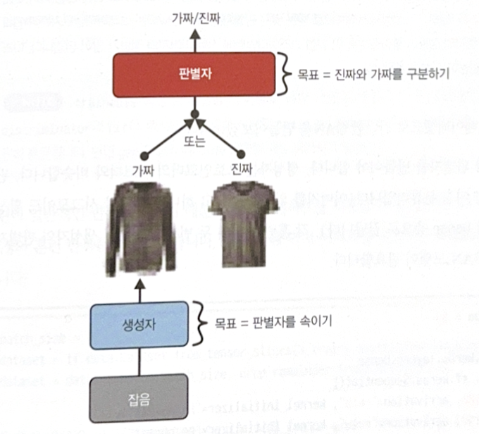
Generative Adversarial Networks(GAN) consists of two NN.
- Generator: Get random distribution(latent coding of output) as input and return data such as image.
- Discriminator: Distinguish whether image is real or fake.

While training, the goal of generator and discriminator is totally opposite.
Each training iteration is composed of two parts.
- Train discriminator. Sample real images(label=1) in train set and merge them with fake images(label=0). Discriminator is trained for a step with the labeled batch. Backpropagation only optimizes weights of discriminator.
- Train generator. Make fake images by using generator. Then, distinguish fake or real by using discriminator, without using real images. Therefore, generator should make fake images which are sufficiently close to real. During this step, weights of discriminator are frozen.
The following is an example of GAN.
# model building
codings_size = 30

Dense = tf.keras.layers.Dense
generator = tf.keras.Sequential([
    tf.keras.layers.Input(shape=(codings_size,)),
    Dense(100, activation='relu', kernel_initializer='he_normal'),
    Dense(150, activation='relu', kernel_initializer='he_normal'),
    Dense(28 * 28, activation='sigmoid'),
    tf.keras.layers.Reshape([28, 28])
])

discriminator = tf.keras.Sequential([
    tf.keras.layers.Flatten(input_shape=[28, 28]),
    Dense(150, activation='relu', kernel_initializer='he_normal'),
    Dense(100, activation='relu', kernel_initializer='he_normal'),
    Dense(1, activation='sigmoid')
])

gan = tf.keras.Sequential([generator, discriminator])

# compiling
discriminator.compile(loss='binary_crossentropy', optimizer='rmsprop')
discriminator.trainable = False     # freeze discriminator
gan.compile(loss='binary_crossentropy', optimizer='rmsprop')

# dataset making
batch_size = 32
dataset = tf.data.Dataset.from_tensor_slices(X_train).shuffle(buffer_size=1000)
dataset = dataset.batch(batch_size, drop_remainder=True).prefetch(1)

# Customized train iteration. Impossible to use fit() method
def train_gan(gan, dataset, batch_size, codings_size, n_epochs):
    generator, discriminator = gan.layers
    for epoch in range(n_epochs):
        for X_batch in dataset:
            # step 1: train discriminator
            noise = tf.random.normal(shape=[batch_size, codings_size])
            generated_images = generator(noise)
            X_fake_and_real = tf.concat([generated_images, X_batch], axis=0)
            y1 = tf.constant([[0.]] * batch_size + [[1.]] * batch_size)
            discriminator.train_on_batch(X_fake_and_real, y1)
            # step 2: train generator
            noise = tf.random.normal(shape=[batch_size, codings_size])
            y2 = tf.constant([[1.]] * batch_size)
            gan.train_on_batch(noise, y2)

train_gan(gan, dataset, batch_size, codings_size, n_epochs=5)
Difficulties of Training GAN
Nash equilibrium is the ultimate goal of GAN. At the state, generator generates images which are perfectly same as real, so the only choice of discriminator is to making a guess.
However, reaching Nash equilibrium is difficult. There are some difficulties while training GAN.
- Mode collapse: Diversity of outputs from generators decreased. It happens when generator only makes images which are easy to cheat discriminator. At the moment, both generator and discriminator will forget to create(or distinguish) other types of images.
- Unstable parameters: As generator and discriminator affects each other, variation of parameters are unstable. To solve this, RMSProp is used instead of Nadam.
There are some solutions for mode collapse.
- Experience replay: In each iteration, store images from generator at reproductive buffer. Train discriminator with real and fake images from buffer(not directly from generator).
- Mini-batch discrimination: Measure the similarity across batches. Discriminator can avoid batches with low diversity.
Deep Convolutional GAN
Deep convolutional GAN(DCGAN) has characteristics as follows.
- Pooling (in discriminator) is changed to stride conv. Pooing (in generator) is changed to transpose conv.
- Batch normalization in both discriminator and generator (except output of generator and input of discriminator).
- Remove fully connected hidden layer to stack deeply.
- All layers of generator use ReLU except tanh is mandatory.
- All layers of discriminator use LeakyReLU.
The following is an implementation of DCGAN. Before training, input shape should be scaled.
codings_size = 100

generator = tf.keras.Sequential([
    tf.keras.layers.Dense(7 * 7 * 128, input_shape=[codings_size]),
    tf.keras.layers.Reshape([7, 7, 128]),
    tf.keras.layers.BatchNormalization(),
    tf.keras.layers.Conv2DTranspose(64, kernel_size=5, strides=2, padding='same', activation='relu'),
    tf.keras.layers.BatchNormalization(),
    tf.keras.layers.Conv2DTranspose(1, kernel_size=5, strides=2, padding='same', activation='tanh'),
])
discriminator = tf.keras.Sequential([
    tf.keras.layers.Conv2D(64, kernel_size=5, strides=2, padding='same', activation=tf.keras.layers.LeakyReLU(0.2), input_shape=[28, 28, 1]),
    tf.keras.layers.Dropout(0.4),
    tf.keras.layers.Conv2D(128, kernel_size=5, strides=2, padding='same', activation=tf.keras.layers.LeakyReLU(0.2)),
    tf.keras.layers.Dropout(0.4),
    tf.keras.layers.Flatten(),
    tf.keras.layers.Dense(1, activation='sigmoid')
])
gan = tf.keras.Sequential([generator, discriminator])
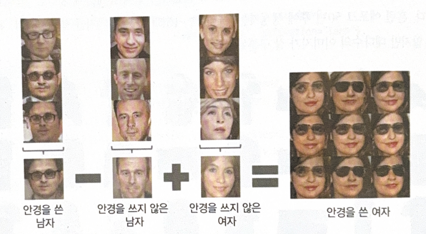
DCGAN can learn meaningful latent representations. It can make images which are very similar to real!

ProGAN
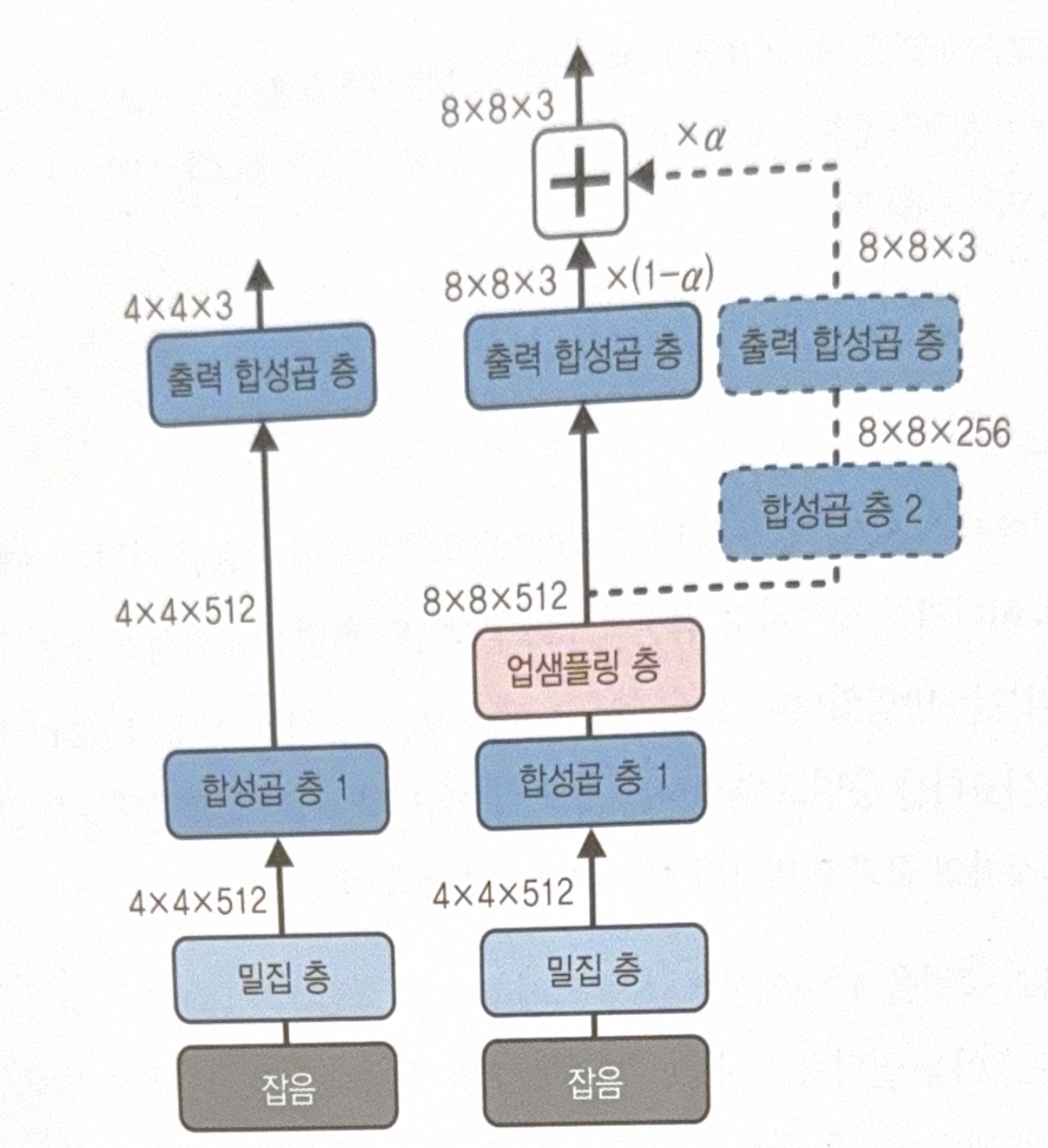
ProGAN uses techniques similar to stacked autoencoder. It makes small image in the early stage, and gradually generates large image by adding conv layer to generator and discriminator.
The following is a structure of ProGAN.

Left part shows the generation of image by using GAN. Right part shows the process of upscaling.
There are some important points in the right part.
- Original output layer is faded-out and two new conv layer are gradually faded-in. To implement this, weight $\alpha$ is used.
- All conv layer uses ‘same’ stride 1. Height and width of input is maintained.
There are some methods to make diverse outputs and training stable.
- Mini-batch std layer: Added to the near of discriminator. As low std means low diversity, this will help discriminator not to be cheated by that kind of batch.
- Same learning speed(rate): Initialize all weights with normal distribution, instead of He initialization. During runtime, downscale weights by using factor in He initialization.
- Pixel-wise normalization layer: Added right after the generator conv layer. This prevents the exploding of activation value.
All images, except those with separate source indications, are excerpted from lecture materials.

댓글남기기