[Hands-On ML] 17. Autoencoders, GANs, and Diffusion Models - 2

Convolutional Autoencoder

When handling image, conv layer will work better. To make an autoencoder for image, we have to make convolutional autoencoder. Encoder reduces the spatial dim(height and width), and increase depth(# of feature maps). Decoder performs the reverse process.

The following is an example of convolutional autoencoder.

conv_encoder = tf.keras.Sequential([
    tf.keras.layers.Reshape([28, 28, 1], input_shape=[28, 28]),
    tf.keras.layers.Conv2D(16, 3, padding='same', activation='relu'),
    tf.keras.layers.MaxPool2D(pool_size=2),
    tf.keras.layers.Conv2D(32, 3, padding='same', activation='relu'),
    tf.keras.layers.MaxPool2D(pool_size=2),
    tf.keras.layers.Conv2D(64, 3, padding='same', activation='relu'),
    tf.keras.layers.MaxPool2D(pool_size=2),
    tf.keras.layers.Conv2D(30, 3, padding='same', activation='relu'),
    tf.keras.layers.GlobalAvgPool2D(),
])
conv_decoder = tf.keras.Sequential([
    tf.keras.layers.Dense(3 * 3 * 16),
    tf.keras.layers.Reshape((3, 3, 16)),
    tf.keras.layers.Conv2DTranspose(32, 3, strides=2, activation='relu'),
    tf.keras.layers.Conv2DTranspose(16, 3, strides=2, activation='relu', padding='same'),
    tf.keras.layers.Conv2DTranspose(1, 3, strides=2, padding='same'),
    tf.keras.layers.Reshape([28, 28])
])
conv_ae = tf.keras.Sequential([conv_encoder, conv_decoder])

Denoising Autoencoder

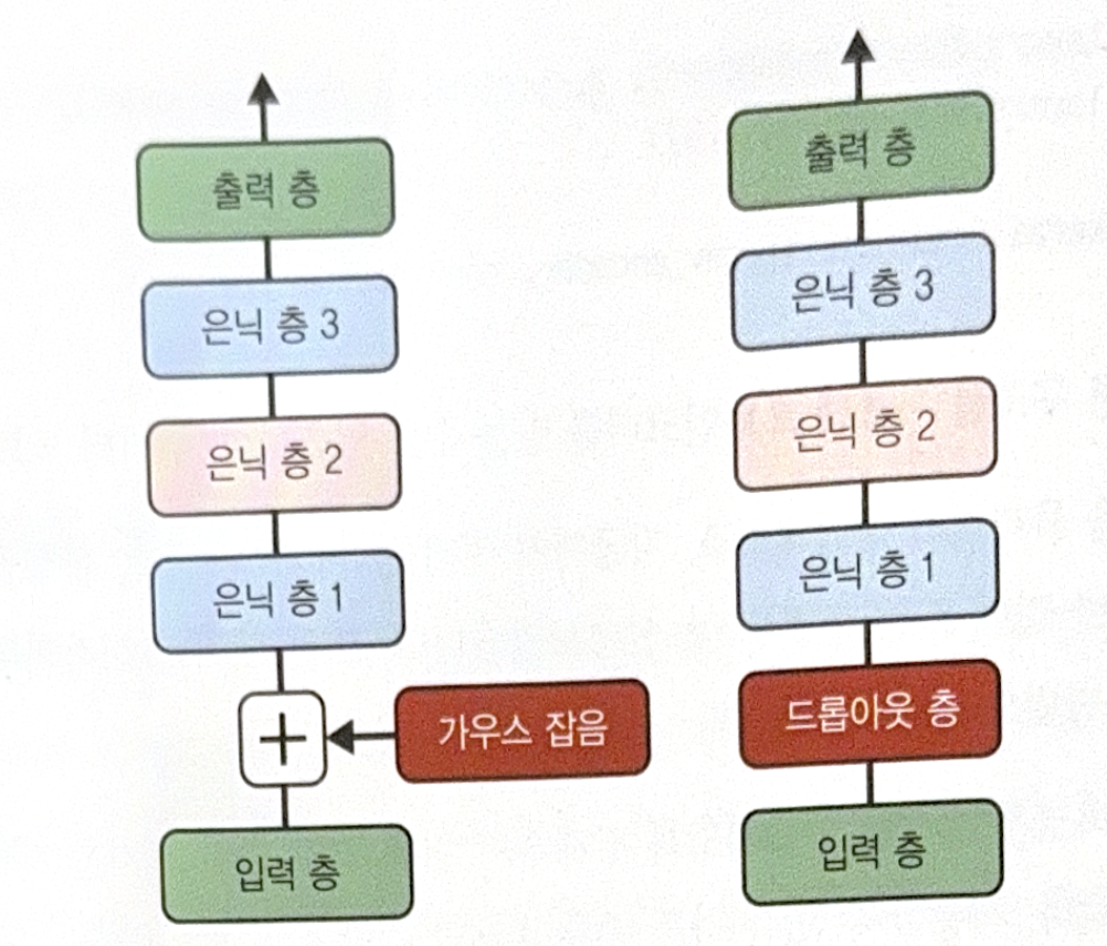
By adding noise to inputs, we can force autoencoder to learn useful features. Add noise first, and then autoencoder will try to remove noise.

There are two ways to make denoising autoencoder.

1. Add Gaussian noise to input.
2. Randomly turn off inputs such as dropout.

The following is an example of dropout.

dropout_encoder = tf.keras.Sequential([
    tf.keras.layers.Flatten(input_shape=(28, 28)),
    tf.keras.layers.Dropout(0.5),
    tf.keras.layers.Dense(100, activation='relu'),
    tf.keras.layers.Dense(30, activation='relu'),
])
dropout_decoder = tf.keras.Sequential([
    tf.keras.layers.Dense(100, activation='relu'),
    tf.keras.layers.Dense(28 * 28),
    tf.keras.layers.Reshape([28, 28])
])
dropout_ae = tf.keras.Sequential([dropout_encoder, dropout_decoder])

Sparsity Autoencoder

By adding appropriate term to cost function, we can decrease the number of activated neurons in a coding layer. Then, the autoencoder should express inputs in a small combination of neurons, and therefore, useful properties will be taught.

The following is a simple way to implement sparsity autoencoder. Use sigmoid function and large coding layer. l1 regularization is also added to the activation of coding layer.

sparse_l1_encoder = tf.keras.Sequential([
    tf.keras.layers.Flatten(input_shape=(28, 28)),
    tf.keras.layers.Dense(100, activation='relu'),
    tf.keras.layers.Dense(300, activation='sigmoid'),
    tf.keras.layers.ActivityRegularization(l1=1e-4)
])
sparse_l1_decoder = tf.keras.Sequential([
    tf.keras.layers.Dense(100, activation='relu'),
    tf.keras.layers.Dense(28 * 28),
    tf.keras.layers.Reshape([28, 28])
])
sparse_l1_ae = tf.keras.Sequential([sparse_l1_encoder, sparse_l1_decoder])

Another method is to impose penalty to the model whose coding layer’s sparsity is different from the target’s one. To do this, we have to calculate average activation of each neuron in coding layer for whole train batch.

By knowing the average activation, we can add sparsity loss to the cost function in order to give a penalty to insufficiently(or overly) activated neuron. Instead of MSE, we can use Kullback-Leibler divergence.

\[D_{KL}(P || Q) = \sum_{i}{P(i) \log{\frac{P(i)}{Q(i)}}}\]

Here, we measure divergence between the objective probability p and real probability q.

\[D_{KL}(p || q) = p \log{\frac{p}{q}} + (1-p) \log{\frac{1-p}{1-q}}\]

After calculating the sparsity loss, add all loss to the result of the cost function. Weight parameter could be multiplied to the sparsity loss to control the relative importance between sparsity loss and reconstruction loss.

To implement KL divergence, customized regularization is needed. For more information, see ‘Go for Codes’.

Variational Autoencoder

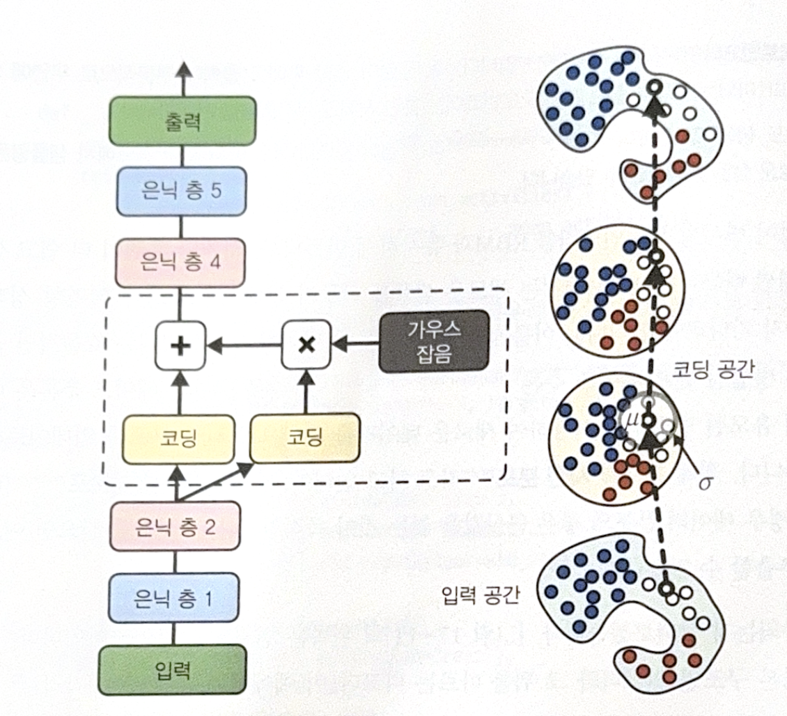
Variational autoencoder has significant difference as follows.

• Probabilistic autoencoder: Output is partially determined by chance even after training.
• Generative autoencoder: Be able to generate new samples similar to sampled in train set.

Variational autoencoder performs variational Bayesian inference, which is an efficient approximate Bayesian inference method. Bayesian inference means updating probability distribution based on new data using Bayesian-derived formulas. Updated distribution is called posterior, and the original distribution is called prior.

The following is a structure of variational autoencoder.

1. Encoder makes ‘mead coding’ $\mu$, and std $\sigma$.
2. Actual coding is randomly sampled in normal distribution, where mean is $\mu$, and std is $\sigma$.
3. Decoder decodes sampled coding as usual.

Whether the input has too complex distribution, variational autoencoder makes coding simple which seems to be sampled in normal distribution. Thanks to the concept, generating a new sample is also easy, just randomly sample in normal distribution!

Cost function is composed of two parts. One is general reconstruction loss. The other is latent loss, which forces the autoencoder to have coding, similar to the one that is sampled from normal distribution. Latent loss looks as a follow.

\[\mathcal{L} = - \frac{1}{2} \sum_{i=1}^{n}{[1 + \log{(\sigma_i^2)} - \sigma_i^2 - \mu_i^2]}\]

n is a dim of coding, $\mu_i$ and $\sigma_i$ are mean and std of ith coding element.

There is also a variation of the loss. It is stable and fast.

\[\mathcal{L} = - \frac{1}{2} \sum_{i=1}^{n}{[1 + \gamma_i - exp(\gamma_i) - \mu_i^2]}, \quad \gamma = \log{(\sigma^2)}\]

For specific code implementation(variational model and sample generation), see ‘Go for Codes’.

Go for Codes

All images, except those with separate source indications, are excerpted from lecture materials.