[Hands-On ML] 15. Processing Sequences Using RNNs and CNNs - 1

Recurrent Neural Network

Recurrent Neural Network(RNN) is appropirate to predict the future from time series data. RNN can handle arbitrary length sequence, so it is useful to auto-translation, speech to text, natural language processing.

RNN is not the only NN that can handle sequence data. CNN also works well.

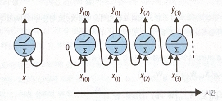
RNN(left image) is similar to feed forward NN, but the difference is that there are recurrent connections. For each time step t, a recurrent neuron gets $\bf{x_{(t)}}$ and $\hat{y}_{(t-1)}$, the output of prior time step, as an input. The RNN can be represented with respect to time, which is called ‘unrolling the nerwork through time’.

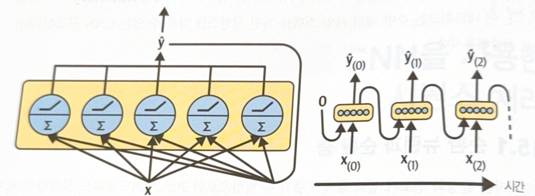
The layer of RNN could be represented as a following image.

By applying vectorization, the output vector of recurrent layer could be written as a follow.

\[\bf{\hat{y}_{(t-1)}} = \phi (\bf{W_x^T x_{(t)} + W_{\hat{y}}^T \hat{y}_{(t-1)} + b})\]

We can also make all inputs to matrix $\bf{X_{(t)}}$ and calculate all output of a recurrent layer for a mini-batch at once.

\[\bf{\hat{Y}_{(t-1)}} = \phi (\bf{X_{(t)} W_x + \hat{Y}_{(t-1)} W_{\hat{y}} + b}) = \phi (\bf{[X_{(t)} \hat{Y}_{(t-1)}] W + b}), \text{where, } W = \begin{bmatrix}W_x\\W_{\hat{y}}\\ \end{bmatrix}\]

At first time step t=0, the former output is assumed as 0.

Memory Cell

A component of NN which preserves a state across time steps are called memory cell. A recurrent layer is a very basic cell that can learn about 10 steps.

Generally, the state of cell at time step t, $\bf{h_{(t)}}$, is a function for an input of the time step and the state of the former time step, $\mathbf{h_{(t)}} = f(\mathbf{x_{(t)}, h_{(t-1)}})$.

Types of RNN according to input and output shape

RNN could be classified into 4 types according to input and output shape.

1. Sequence-to-Sequence Network (top-left on image)
   Useful to predict time series data.
   e.g. If you input recent N days data, the nerwork will predict N-1 to tomorrow.

2. Sequence-to-Vector Network (top-right on image)
   Inject input sequence to NN and ignore all outputs, but the last one.
   e.g. Inject a movie review, print a sentiment score.

3. Vector-to-Sequence Network (bottom-left on image)
   Repeatedly input one vector to NN for each time step, output one sequence.
   e.g. Input a image and output a caption.

4. Encoder and Decoder (bottom-right on image)
   Encoder(Sequence-to-Vector) are followed by a decoder(Vector-to-Sequence).
   e.g. Translation. Encoder will make a sentence to vector, and decoder will make the vector to sequence of another language. This NN works better than simple RNN, because it considers the context.

Train RNN

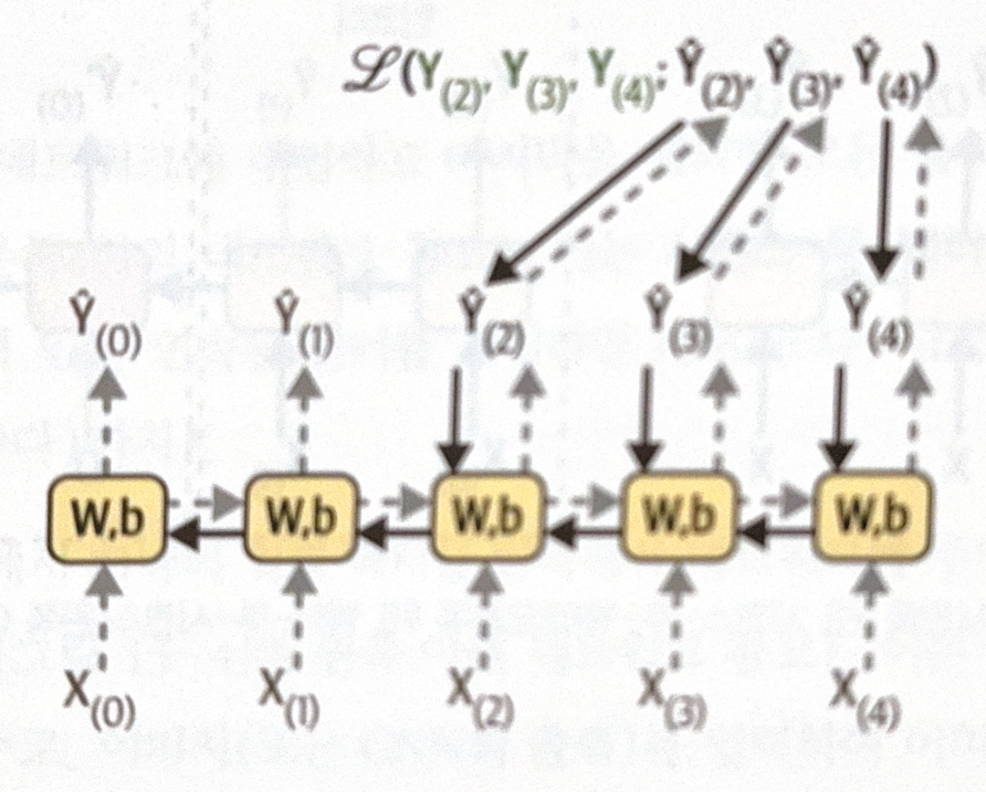
Backpropagation could also applied to RNN. Before apply backprop, we will first unroll the nerwork through time. This tactic is called BPTT(BackPropagation Through Time).

In real process, RNN class does not unroll the NN. Just think this way, and it will make it easy to understand.

Forwardprop is marked in gray dotted line, and backprop is marked in black line. As represented, some output could be ignored. The ignored outputs will not get gradients. Same W, and b is used for each time step, and they will be adjucted multiple times during backprop.

Predict Time Series

Here, I used dataset from Chicago Transit Authority. The purpose is to predict the number of tomorrow passengers.

For specific codes, look at Go for Codes. Let’s look at some important points.

• Seasonality
  The dataset has seasonality, which means that similar pattern is repeated. If the pattern is strong, just repeating the pattern for prediction will work fine. This is called naive forecasting,and it is sometimes more powerful than any other methods.

• Differencing
  Differencing means getting a difference between two time series. It is used for naive forecasting.
  After differencing, seasonality and trends could be removed, and the time series would be a stationary time series, which is easier to analyze.

• Autocorrelation
  If delayed time series has a correlation to itself, it is called autocorrelation.

ARMA model

ARMA(Auroregressive Moving Average) gets a prediction from simple weighted sum of delayed values, and modify the prediction by adding moving average.

\[\displaystyle \hat{y}_{(t)} = \sum_{i=1}^{p}{\alpha_i y_{(t-1)}} + \sum_{i=1}^{q}{\theta_i \epsilon_{(t-1)}}, \text{where } \epsilon_{(t)} = y_{(t)} - \hat{y}_{(t-1)}\]

The first sum is about weighted sum of delayed values, and the second sum is about moving average.

The model assumes that the dataset is stationary time series. Therefore, if the dataset is not a stationary time series, apply differencing first. From succesive d times differencing, we can get dth derivative, which could remove dth mutivariative trends. Hyperparameter d is order of integration.

In ARIMA(Auroregressive Integrated Moving Average), differencing is the core component. The model performs d times differencing to make a stationary time series, and apply ARMA. The value which wat subtracted from differencing should be added to the final prediction.

Seasonal ARIMA(SARIMA) additionally models a seasonal term. It has total 7 parameters, p, d, q for ARIMA, P, D, Q for seasonal pattern, and s for an interval of seasonal pattern.

When using ARIMA class, set asfreq() for a frequency. If not, ARIMA class will automatically predict the frequency, and warning will be printed.

The 7 hyperparameters could be searched by grid search. Good p, q, P, Q values are usually small, and good d, D is 0 or 1. For s, it depens on the pattern of dataset (in this example, it is 7 because it has a strong weekly seasonality).

Go for Code

별도의 출처 표시가 있는 이미지를 제외한 모든 이미지는 강의자료에서 발췌하였음을 밝힙니다.