[Hands-On ML] 14. Deep Computer Vision Using Convolutional Neural Networks - 1

Convolutional Layer

The most important component of Convolutional Neural Network(CNN) is a convolutional layer. A neuron in the first convolutional layer is only connected to the pixel in receptive field. This kind of hierarchical structure is continued.

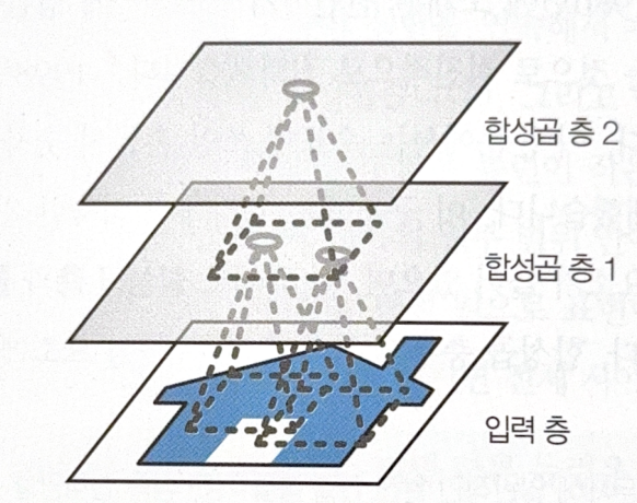
There is no need to flatten inputs to 1D array.

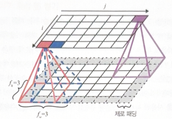
A neuron at row i, column j in a layer is connected to the prior layer’s i to $i+f_h-1$ rows and j to $j+f_w-1$ columns outputs.

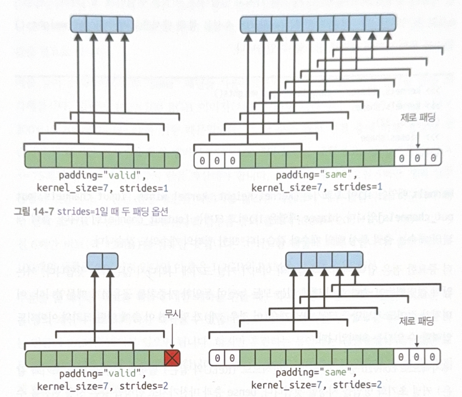
As multiple number of outputs are merged into a unit, size(shape) of a layer would be smaller than the prior one. To prevent this, zeros will be added around the inputs. This is called zero paddings.

Stride is a step size between a receptive field. The following is an example of stride 2. You can check that the reception field moves 2 steps at a time.

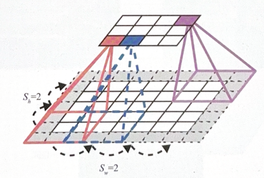
When using a stride, neuron $_{i, j}$ of upper layer is connected to the lower layer’s

$i \times s_h$ to $i \times s_h + f_h - 1$ rows,

$j \times s_w$ to $j \times s_w + f_w - 1$ columns ($s_h$ is a height of a stride, $s_w$ is a width of a stride).

Filter

Filter(or kernel) is a set of weights, which can emphasize characteristics of an image. The followings are examples of two different filters, one is for vertical, and the other is for horizontal.

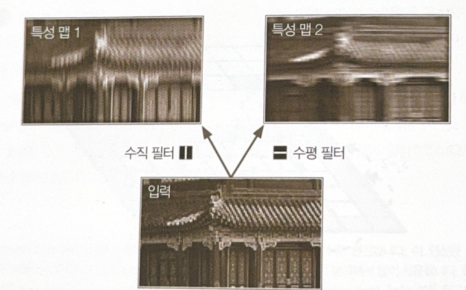
One filter applyed for a layer can make a feature map, with an emphasized characteristic.

Filter are not needed to be defined manually. CNN will automatically find the most useful filter for the problem.

CNN uses multiple filters and stack the results(feature maps). Therefore, the structure can be visualized in 3D.

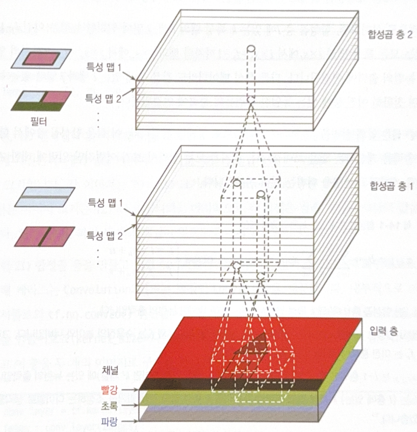
In one feature map, every neuron shares the same parameters(weighs and biases), but neurons in different feature maps use different parameters.

Input images sometimes have sub layers for a color channel, such as RGB(3 sub layers). Other types of channel like infrared layer could also exist.

A neuron$_{i, j}$ in a feature map $k$ of CNN layer $l$ are connected to the outputs of

$i \times s_h$ to $i \times s_h + f_h - 1$ rows,

$j \times s_w$ to $j \times s_w + f_w - 1$ columns

in all feature maps of layer $l-1$.

CNN with keras

When making a 2D CNN layer, do as a follow.

conv_layer = tf.keras.layers.Conv2D(filters=32, kernel_size=7)
fmaps = conv_layer(images)

The layer above has 32 filters, with 7 by 7 shape.

Name ‘2D’ means spatial dimension, height and width. The input for the layer is 4D, (# sample images, height, width, # channels)

Conv2D layer does not use zero padding(padding='valid'). If you want to maintain the size, set padding='same'. However, stride 2+ cannot maintain the size.

Pooling Layer

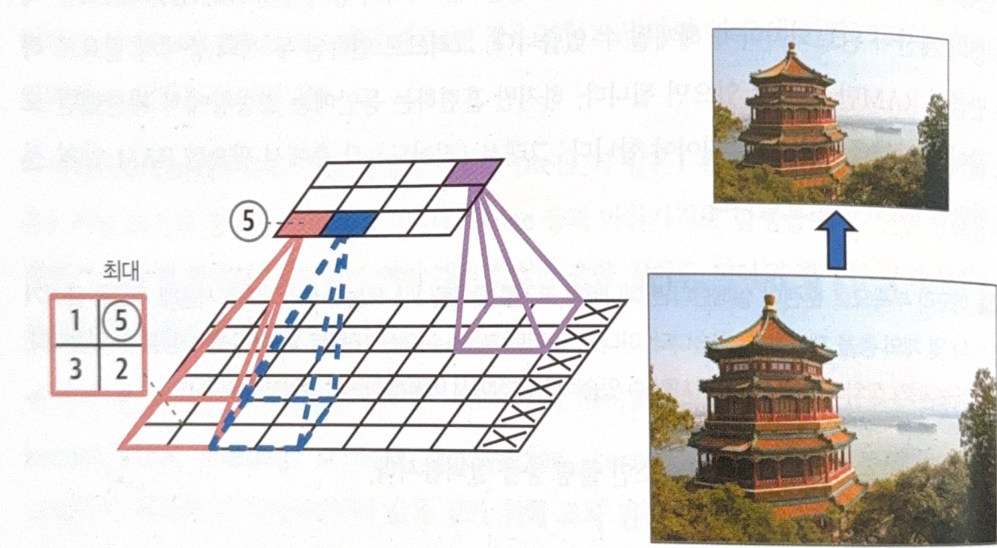
Pooling layer is for making a subsample of an input image to reduce the number of parameters. A pooling layer is similar to CNN layer, with size, stride and padding shape. However, a pooling layer doesn’t have weights.

There are two types of pooling.

• Max Pooling: Choose the max value in a receptive field.
• Average Pooling: Average values in a receptive field.

Only one value is delievered the next layer, and the others are removed.

The following is an example of 2 by 2 max pooling.

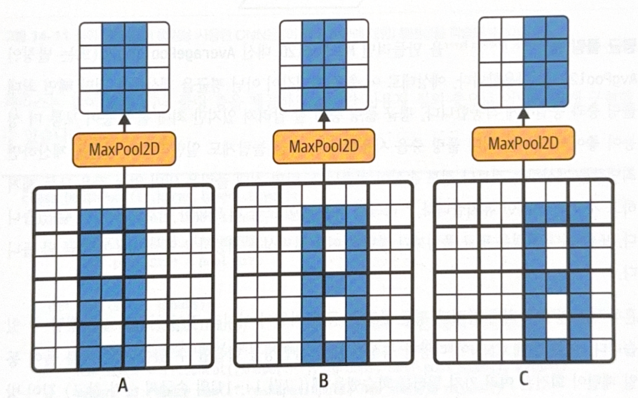
Max pooling provides invariance. Small translation of inputs might not be reflected in the output.

Implementing max pooling is keras is easy.

max_pool = tf.keras.layers.MaxPool2D(pool_size=2)

For average pooling, use AvgPool2D.

Max pooling could be performed with respect to depth, not a space. This could learn the invariance of various features. For example, depthwise max pooling makes the same output no matter how much the input image are rotated.

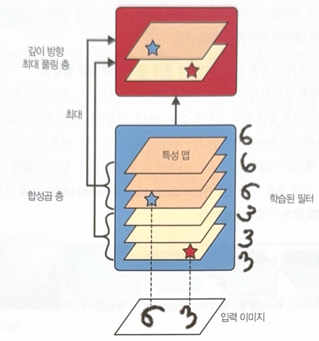
Keras doesn’t provide depthwise max pooling, so you should implement manually with class.

# depthwise pooling
class DepthPool(tf.keras.layers.Layer):
    def __init__(self, pool_size=2, **kwargs):
        super().__init__(**kwargs)
        self.pool_size = pool_size

    def call(self, inputs):
        shape = tf.shape(inputs)
        groups = shape[-1] // self.pool_size
        new_shape = tf.concat([shape[:-1], [groups, self.pool_size]], axis=0)
        return tf.reduce_max(tf.reshape(inputs, new_shape), axis=-1)

There is also a Global Average Pooling Layer. The layer calculates the average of each feature map. One value for one feature map! Very destructive, but useful right before the output layer.

# method 1
global_avg_pool = tf.keras.layers.GlobalAvgPool2D()


# method 2
global_avg_pool = tf.keras.layers.Lambda(
    lambda X: tf.reduce_mean(X, axis=[1, 2])
)

Go for Code

All images, except those with separate source indications, are excerpted from lecture materials.